5 Data Manipulation with dplyr
https://learn.datacamp.com/courses/data-manipulation-with-dplyr
Main functions and concepts covered in this BP chapter:
select()filter()arrange()mutate()count()group_by()ungroup()slice_min/max()summarize()transmute()
Packages used in this chapter:
## Load all packages used in this chapter
library(tidyverse) #includes dplyr, ggplot2, and other common packages
## ── Attaching packages ─────────────────────────────────────── tidyverse 1.3.2 ──
## ✔ ggplot2 3.4.0 ✔ purrr 0.3.5
## ✔ tibble 3.1.8 ✔ dplyr 1.0.10
## ✔ tidyr 1.2.1 ✔ stringr 1.5.0
## ✔ readr 2.1.3 ✔ forcats 0.5.2
## ── Conflicts ────────────────────────────────────────── tidyverse_conflicts() ──
## ✖ dplyr::filter() masks stats::filter()
## ✖ dplyr::lag() masks stats::lag()library(Lock5Data)Datasets used in this chapter:
## Load datasets used in this chapter
counties <- read_rds("data/counties.rds")
babynames <- read_rds("data/babynames.rds")
Tip: don’t forget the pipe (%>%) between each step
5.1 Transforming Data with dplyr
select(), which pulls only certain variables from a larger data set, arrange(), which organizes the data set based on a variable, filter(), which filters out certain values, and mutate(), which changes certain variables.
#Selecting only the variables we want to work with
happyplanet <- HappyPlanetIndex %>%
  select(Country, Region, Happiness, LifeExpectancy, Footprint, GDPperCapita, Population)

#Arranging data in descending order based on population
happyplanet %>%
  arrange(desc(Population))
## Country Region Happiness LifeExpectancy Footprint
## 1 China 6 6.7 72.5 2.1
## 2 India 5 5.5 63.7 0.9
## 3 United States of America 2 7.9 77.9 9.4
## 4 Indonesia 6 5.7 69.7 0.9
## 5 Brazil 1 7.6 71.7 2.4
## 6 Pakistan 5 5.6 64.6 0.8
## 7 Bangladesh 5 5.3 63.1 0.6
## 8 Russia 7 5.9 65.0 3.7
## 9 Nigeria 4 4.8 46.5 1.3
## 10 Japan 6 6.8 82.3 4.9
## 11 Mexico 1 7.7 75.6 3.4
## 12 Philippines 6 5.5 71.0 0.9
## 13 Vietnam 6 6.5 73.7 1.3
## 14 Germany 2 7.2 79.1 4.2
## 15 Ethiopia 4 4.0 51.8 1.4
## 16 Egypt 3 6.7 70.7 1.7
## 17 Turkey 3 5.5 71.4 2.7
## 18 Iran 3 5.6 70.2 2.7
## 19 Thailand 6 6.3 69.6 2.1
## 20 France 2 7.1 80.2 4.9
## 21 United Kingdom 2 7.4 79.0 5.3
## 22 Congo, Dem. Rep. of the 4 3.9 45.8 0.6
## 23 Italy 2 6.9 80.3 4.8
## 24 Korea 6 6.3 77.9 3.7
## 25 Burma 5 5.9 60.8 1.1
## 26 Ukraine 7 5.3 67.7 2.7
## 27 South Africa 4 5.0 50.8 2.1
## 28 Colombia 1 7.3 72.3 1.8
## 29 Spain 2 7.6 80.5 5.7
## 30 Argentina 1 7.1 74.8 2.5
## 31 Tanzania 4 2.4 51.0 1.1
## 32 Poland 7 6.5 75.2 4.0
## 33 Sudan 4 4.5 57.4 2.4
## 34 Kenya 4 3.7 52.1 1.1
## 35 Algeria 3 5.6 71.7 1.7
## 36 Canada 2 8.0 80.3 7.1
## 37 Morocco 3 5.6 70.4 1.1
## 38 Iraq 3 5.4 57.7 1.3
## 39 Uganda 4 4.5 49.7 1.4
## 40 Peru 1 5.9 70.7 1.6
## 41 Nepal 5 5.3 62.6 0.8
## 42 Venezuela 1 6.9 73.2 2.8
## 43 Uzbekistan 7 6.0 66.8 1.8
## 44 Malaysia 6 6.6 73.7 2.4
## 45 Saudi Arabia 3 7.7 72.2 2.6
## 46 Ghana 4 4.7 59.1 1.5
## 47 Romania 7 5.9 71.9 2.9
## 48 Yemen 3 5.2 61.5 0.9
## 49 Mozambique 4 3.8 42.8 0.9
## 50 Australia 2 7.9 80.9 7.8
## 51 Sri Lanka 5 5.4 71.6 1.0
## 52 Syria 3 5.9 73.6 2.1
## 53 Madagascar 4 3.7 58.4 1.1
## 54 Cameroon 4 3.9 49.8 1.3
## 55 Netherlands 2 7.7 79.2 4.4
## 56 Chile 1 6.3 78.3 3.0
## 57 Angola 4 4.3 41.7 0.9
## 58 Kazakhstan 7 6.1 65.9 3.4
## 59 Cambodia 6 4.9 58.0 0.9
## 60 Burkina Faso 4 3.6 51.4 2.0
## 61 Niger 4 3.8 55.8 1.6
## 62 Malawi 4 4.4 46.3 0.5
## 63 Zimbabwe 4 2.8 40.9 1.1
## 64 Ecuador 1 6.4 74.7 2.2
## 65 Guatemala 1 7.4 69.7 1.5
## 66 Senegal 4 4.5 62.3 1.4
## 67 Mali 4 3.8 53.1 1.6
## 68 Zambia 4 4.3 40.5 0.8
## 69 Cuba 1 6.7 77.7 1.8
## 70 Greece 2 6.8 78.9 5.9
## 71 Portugal 2 5.9 77.7 4.4
## 72 Belgium 2 7.6 78.8 5.1
## 73 Czech Republic 7 6.9 75.9 5.4
## 74 Chad 4 5.4 50.4 1.7
## 75 Hungary 7 5.7 72.9 3.5
## 76 Tunisia 3 5.9 73.5 1.8
## 77 Belarus 7 5.8 68.7 3.9
## 78 Dominican Republic 1 7.6 71.5 1.5
## 79 Haiti 1 5.2 59.5 0.5
## 80 Rwanda 4 4.2 45.2 0.8
## 81 Bolivia 1 6.5 64.7 2.1
## 82 Sweden 2 7.9 80.5 5.1
## 83 Guinea 4 4.0 54.8 1.3
## 84 Benin 4 3.0 55.4 1.0
## 85 Azerbaijan 7 5.3 67.1 2.2
## 86 Austria 2 7.8 79.4 5.0
## 87 Burundi 4 2.9 48.5 0.8
## 88 Bulgaria 7 5.5 72.7 2.7
## 89 Serbia 7 6.0 73.6 2.6
## 90 Switzerland 2 7.7 81.3 5.0
## 91 Israel 3 7.1 80.3 4.8
## 92 Honduras 1 7.0 69.4 1.8
## 93 Hong Kong 6 7.2 81.9 5.7
## 94 El Salvador 1 6.7 71.3 1.6
## 95 Tajikistan 7 5.1 66.3 0.7
## 96 Togo 4 2.6 57.8 0.8
## 97 Paraguay 1 6.9 71.3 3.2
## 98 Laos 6 6.2 63.2 1.1
## 99 Sierra Leone 4 3.6 41.8 0.8
## 100 Nicaragua 1 7.1 71.9 2.0
## 101 Denmark 2 8.1 77.9 8.0
## 102 Jordan 3 6.0 71.9 1.7
## 103 Slovakia 7 6.1 74.2 3.3
## 104 Finland 2 8.0 78.9 5.2
## 105 Kyrgyzstan 7 5.0 65.6 1.1
## 106 Norway 2 8.1 79.8 6.9
## 107 Georgia 7 4.3 70.7 1.1
## 108 Croatia 7 6.4 75.3 3.2
## 109 Costa Rica 1 8.5 78.5 2.3
## 110 Singapore 6 7.1 79.4 4.2
## 111 Central African Republic 4 4.0 43.7 1.6
## 112 Ireland 2 8.1 78.4 6.3
## 113 New Zealand 2 7.8 79.8 7.7
## 114 United Arab Emirates 3 7.2 78.3 9.5
## 115 Lebanon 3 4.7 71.5 3.1
## 116 Moldova 7 5.7 68.4 1.2
## 117 Bosnia and Herzegovina 7 5.9 74.5 2.9
## 118 Palestine 3 5.0 72.9 1.5
## 119 Congo 4 3.6 54.0 0.5
## 120 Lithuania 7 5.8 72.5 3.2
## 121 Uruguay 1 6.8 75.9 5.5
## 122 Panama 1 7.8 75.1 3.2
## 123 Albania 7 5.5 76.2 2.2
## 124 Armenia 7 5.0 71.7 1.4
## 125 Mauritania 4 5.0 63.2 1.9
## 126 Jamaica 1 6.7 72.2 1.1
## 127 Mongolia 7 5.7 65.9 3.5
## 128 Kuwait 3 6.7 77.3 8.9
## 129 Latvia 7 5.4 72.0 3.5
## 130 Macedonia 7 5.5 73.8 4.6
## 131 Namibia 4 4.5 51.6 3.7
## 132 Slovenia 7 7.0 77.4 4.5
## 133 Botswana 4 4.7 48.1 3.6
## 134 Estonia 7 5.6 71.2 6.4
## 135 Trinidad and Tobago 1 6.7 69.2 2.1
## 136 Djibouti 4 5.7 53.9 1.5
## 137 Cyprus 2 7.2 79.0 4.5
## 138 Guyana 1 6.5 65.2 2.6
## 139 Bhutan 5 6.1 64.7 1.0
## 140 Luxembourg 2 7.7 78.4 10.2
## 141 Malta 2 7.1 79.1 3.8
## 142 Iceland 2 7.8 81.5 7.4
## 143 Belize 1 6.6 75.9 2.6
## GDPperCapita Population
## 1 6757 1304.50
## 2 3452 1094.58
## 3 41890 296.51
## 4 3843 220.56
## 5 8402 186.83
## 6 2370 155.77
## 7 2053 153.28
## 8 10845 143.15
## 9 1128 141.36
## 10 31267 127.77
## 11 10751 103.09
## 12 5137 84.57
## 13 3071 83.10
## 14 29461 82.47
## 15 1055 75.17
## 16 4337 72.85
## 17 8407 72.07
## 18 7968 69.09
## 19 8677 63.00
## 20 30386 60.87
## 21 33238 60.23
## 22 714 58.74
## 23 28529 58.61
## 24 22029 48.29
## 25 1027 47.97
## 26 6848 47.11
## 27 11110 46.89
## 28 7304 44.95
## 29 27169 43.40
## 30 14280 38.75
## 31 744 38.48
## 32 13847 38.17
## 33 2083 36.90
## 34 1240 35.60
## 35 7062 32.85
## 36 33375 32.31
## 37 4555 30.14
## 38 NA 29.27
## 39 1454 28.95
## 40 6039 27.27
## 41 1550 27.09
## 42 6632 26.58
## 43 2063 26.17
## 44 10882 25.65
## 45 15711 23.12
## 46 2480 22.54
## 47 9060 21.63
## 48 930 21.10
## 49 1242 20.53
## 50 31794 20.40
## 51 4595 19.67
## 52 3808 18.89
## 53 923 18.64
## 54 2299 17.80
## 55 32684 16.32
## 56 12027 16.30
## 57 2335 16.10
## 58 7857 15.15
## 59 2727 13.96
## 60 1213 13.93
## 61 781 13.26
## 62 667 13.23
## 63 2038 13.12
## 64 4341 13.06
## 65 4568 12.71
## 66 1792 11.77
## 67 1033 11.61
## 68 1023 11.48
## 69 6000 11.26
## 70 23381 11.10
## 71 20410 10.55
## 72 32119 10.48
## 73 20538 10.23
## 74 1427 10.15
## 75 17887 10.09
## 76 8371 10.03
## 77 7918 9.78
## 78 8217 9.47
## 79 1663 9.30
## 80 1206 9.23
## 81 2819 9.18
## 82 32525 9.02
## 83 2316 9.00
## 84 1141 8.49
## 85 5016 8.39
## 86 33700 8.23
## 87 699 7.86
## 88 9032 7.74
## 89 NA 7.44
## 90 35633 7.44
## 91 25864 6.92
## 92 3430 6.83
## 93 34833 6.81
## 94 5255 6.67
## 95 1356 6.55
## 96 1506 6.24
## 97 4642 5.90
## 98 2039 5.66
## 99 806 5.59
## 100 3674 5.46
## 101 33973 5.42
## 102 5530 5.41
## 103 15871 5.39
## 104 32153 5.25
## 105 1927 5.14
## 106 41420 4.62
## 107 3365 4.47
## 108 13042 4.44
## 109 10180 4.33
## 110 29663 4.27
## 111 1224 4.19
## 112 38505 4.16
## 113 24996 4.13
## 114 25514 4.10
## 115 5584 4.01
## 116 2100 3.88
## 117 7032 3.78
## 118 1500 3.76
## 119 1262 3.61
## 120 14494 3.41
## 121 9962 3.31
## 122 7605 3.23
## 123 5316 3.15
## 124 4945 3.02
## 125 2234 2.96
## 126 4291 2.65
## 127 2107 2.55
## 128 26321 2.54
## 129 13646 2.30
## 130 7200 2.03
## 131 7586 2.02
## 132 22273 2.00
## 133 12387 1.84
## 134 15478 1.35
## 135 14603 1.32
## 136 2178 0.80
## 137 22699 0.76
## 138 4508 0.74
## 139 3649 0.64
## 140 60228 0.46
## 141 19189 0.40
## 142 36510 0.30
## 143 7109 0.29head(happyplanet)## Country Region Happiness LifeExpectancy Footprint GDPperCapita Population
## 1 Albania 7 5.5 76.2 2.2 5316 3.15
## 2 Algeria 3 5.6 71.7 1.7 7062 32.85
## 3 Angola 4 4.3 41.7 0.9 2335 16.10
## 4 Argentina 1 7.1 74.8 2.5 14280 38.75
## 5 Armenia 7 5.0 71.7 1.4 4945 3.02
## 6 Australia 2 7.9 80.9 7.8 31794 20.40#Only including data where population > 10 million (10)
happybigplanet <- happyplanet %>%
filter(Population > 10)
head(happybigplanet)## Country Region Happiness LifeExpectancy Footprint GDPperCapita Population
## 1 Algeria 3 5.6 71.7 1.7 7062 32.85
## 2 Angola 4 4.3 41.7 0.9 2335 16.10
## 3 Argentina 1 7.1 74.8 2.5 14280 38.75
## 4 Australia 2 7.9 80.9 7.8 31794 20.40
## 5 Bangladesh 5 5.3 63.1 0.6 2053 153.28
## 6 Belgium 2 7.6 78.8 5.1 32119 10.48#Only including data from Western Nations where population > 10 million
happywestnat <- happyplanet %>%
filter(Region == 2, Population > 10)
#Arrange data set in descending order based on happiness
happywestnat %>%
arrange(desc(Happiness))## Country Region Happiness LifeExpectancy Footprint
## 1 Canada 2 8.0 80.3 7.1
## 2 Australia 2 7.9 80.9 7.8
## 3 United States of America 2 7.9 77.9 9.4
## 4 Netherlands 2 7.7 79.2 4.4
## 5 Belgium 2 7.6 78.8 5.1
## 6 Spain 2 7.6 80.5 5.7
## 7 United Kingdom 2 7.4 79.0 5.3
## 8 Germany 2 7.2 79.1 4.2
## 9 France 2 7.1 80.2 4.9
## 10 Italy 2 6.9 80.3 4.8
## 11 Greece 2 6.8 78.9 5.9
## 12 Portugal 2 5.9 77.7 4.4
## GDPperCapita Population
## 1 33375 32.31
## 2 31794 20.40
## 3 41890 296.51
## 4 32684 16.32
## 5 32119 10.48
## 6 27169 43.40
## 7 33238 60.23
## 8 29461 82.47
## 9 30386 60.87
## 10 28529 58.61
## 11 23381 11.10
## 12 20410 10.55head(happywestnat)## Country Region Happiness LifeExpectancy Footprint GDPperCapita Population
## 1 Australia 2 7.9 80.9 7.8 31794 20.40
## 2 Belgium 2 7.6 78.8 5.1 32119 10.48
## 3 Canada 2 8.0 80.3 7.1 33375 32.31
## 4 France 2 7.1 80.2 4.9 30386 60.87
## 5 Germany 2 7.2 79.1 4.2 29461 82.47
## 6 Greece 2 6.8 78.9 5.9 23381 11.10#Mutate data set to add variable for total GDP by multiplying GDP/capita by population
happyplanet <- happyplanet %>%
mutate(total_GDP = GDPperCapita * Population)
head(happyplanet)## Country Region Happiness LifeExpectancy Footprint GDPperCapita Population
## 1 Albania 7 5.5 76.2 2.2 5316 3.15
## 2 Algeria 3 5.6 71.7 1.7 7062 32.85
## 3 Angola 4 4.3 41.7 0.9 2335 16.10
## 4 Argentina 1 7.1 74.8 2.5 14280 38.75
## 5 Armenia 7 5.0 71.7 1.4 4945 3.02
## 6 Australia 2 7.9 80.9 7.8 31794 20.40
## total_GDP
## 1 16745.4
## 2 231986.7
## 3 37593.5
## 4 553350.0
## 5 14933.9
## 6 648597.65.2 Aggregating Data
There are a number of functions you can use to take many observations in your data and summarize them, including count(), group_by(), summarize(), ungroup(), and top_n().
5.2.1 Count
#Using `count()` to see how many countries are in each region and then arranged in descending order
happyplanet %>%
  count(region, sort = TRUE)
## region n
## 1 Sub-Saharan Africa 33
## 2 former Communist countries 27
## 3 Latin America 24
## 4 Western Nations 24
## 5 Middle East 16
## 6 East Asia 12
## 7 South Asia 7#Using `count()` to find number of observations for each country, weighted by population.
happyplanet %>%
count(Country, wt = Population, sort = TRUE)## Country n
## 1 China 1304.50
## 2 India 1094.58
## 3 United States of America 296.51
## 4 Indonesia 220.56
## 5 Brazil 186.83
## 6 Pakistan 155.77
## 7 Bangladesh 153.28
## 8 Russia 143.15
## 9 Nigeria 141.36
## 10 Japan 127.77
## 11 Mexico 103.09
## 12 Philippines 84.57
## 13 Vietnam 83.10
## 14 Germany 82.47
## 15 Ethiopia 75.17
## 16 Egypt 72.85
## 17 Turkey 72.07
## 18 Iran 69.09
## 19 Thailand 63.00
## 20 France 60.87
## 21 United Kingdom 60.23
## 22 Congo, Dem. Rep. of the 58.74
## 23 Italy 58.61
## 24 Korea 48.29
## 25 Burma 47.97
## 26 Ukraine 47.11
## 27 South Africa 46.89
## 28 Colombia 44.95
## 29 Spain 43.40
## 30 Argentina 38.75
## 31 Tanzania 38.48
## 32 Poland 38.17
## 33 Sudan 36.90
## 34 Kenya 35.60
## 35 Algeria 32.85
## 36 Canada 32.31
## 37 Morocco 30.14
## 38 Iraq 29.27
## 39 Uganda 28.95
## 40 Peru 27.27
## 41 Nepal 27.09
## 42 Venezuela 26.58
## 43 Uzbekistan 26.17
## 44 Malaysia 25.65
## 45 Saudi Arabia 23.12
## 46 Ghana 22.54
## 47 Romania 21.63
## 48 Yemen 21.10
## 49 Mozambique 20.53
## 50 Australia 20.40
## 51 Sri Lanka 19.67
## 52 Syria 18.89
## 53 Madagascar 18.64
## 54 Cameroon 17.80
## 55 Netherlands 16.32
## 56 Chile 16.30
## 57 Angola 16.10
## 58 Kazakhstan 15.15
## 59 Cambodia 13.96
## 60 Burkina Faso 13.93
## 61 Niger 13.26
## 62 Malawi 13.23
## 63 Zimbabwe 13.12
## 64 Ecuador 13.06
## 65 Guatemala 12.71
## 66 Senegal 11.77
## 67 Mali 11.61
## 68 Zambia 11.48
## 69 Cuba 11.26
## 70 Greece 11.10
## 71 Portugal 10.55
## 72 Belgium 10.48
## 73 Czech Republic 10.23
## 74 Chad 10.15
## 75 Hungary 10.09
## 76 Tunisia 10.03
## 77 Belarus 9.78
## 78 Dominican Republic 9.47
## 79 Haiti 9.30
## 80 Rwanda 9.23
## 81 Bolivia 9.18
## 82 Sweden 9.02
## 83 Guinea 9.00
## 84 Benin 8.49
## 85 Azerbaijan 8.39
## 86 Austria 8.23
## 87 Burundi 7.86
## 88 Bulgaria 7.74
## 89 Serbia 7.44
## 90 Switzerland 7.44
## 91 Israel 6.92
## 92 Honduras 6.83
## 93 Hong Kong 6.81
## 94 El Salvador 6.67
## 95 Tajikistan 6.55
## 96 Togo 6.24
## 97 Paraguay 5.90
## 98 Laos 5.66
## 99 Sierra Leone 5.59
## 100 Nicaragua 5.46
## 101 Denmark 5.42
## 102 Jordan 5.41
## 103 Slovakia 5.39
## 104 Finland 5.25
## 105 Kyrgyzstan 5.14
## 106 Norway 4.62
## 107 Georgia 4.47
## 108 Croatia 4.44
## 109 Costa Rica 4.33
## 110 Singapore 4.27
## 111 Central African Republic 4.19
## 112 Ireland 4.16
## 113 New Zealand 4.13
## 114 United Arab Emirates 4.10
## 115 Lebanon 4.01
## 116 Moldova 3.88
## 117 Bosnia and Herzegovina 3.78
## 118 Palestine 3.76
## 119 Congo 3.61
## 120 Lithuania 3.41
## 121 Uruguay 3.31
## 122 Panama 3.23
## 123 Albania 3.15
## 124 Armenia 3.02
## 125 Mauritania 2.96
## 126 Jamaica 2.65
## 127 Mongolia 2.55
## 128 Kuwait 2.54
## 129 Latvia 2.30
## 130 Macedonia 2.03
## 131 Namibia 2.02
## 132 Slovenia 2.00
## 133 Botswana 1.84
## 134 Estonia 1.35
## 135 Trinidad and Tobago 1.32
## 136 Djibouti 0.80
## 137 Cyprus 0.76
## 138 Guyana 0.74
## 139 Bhutan 0.64
## 140 Luxembourg 0.46
## 141 Malta 0.40
## 142 Iceland 0.30
## 143 Belize 0.29#Using `mutate()` and `count()` to find the countries with the highest total GDP
happyplanet %>%
mutate(total_gdp = GDPperCapita * Population) %>%
count(Country, wt = total_gdp, sort = TRUE)## Country n
## 1 United States of America 12420803.90
## 2 China 8814506.50
## 3 Japan 3994984.59
## 4 India 3778490.16
## 5 Germany 2429648.67
## 6 United Kingdom 2001924.74
## 7 France 1849595.82
## 8 Italy 1672084.69
## 9 Brazil 1569745.66
## 10 Russia 1552461.75
## 11 Spain 1179134.60
## 12 Mexico 1108320.59
## 13 Canada 1078346.25
## 14 Korea 1063780.41
## 15 Indonesia 847612.08
## 16 Australia 648597.60
## 17 Turkey 605892.49
## 18 Argentina 553350.00
## 19 Iran 550509.12
## 20 Thailand 546651.00
## 21 Netherlands 533402.88
## 22 Poland 528539.99
## 23 South Africa 520947.90
## 24 Philippines 434436.09
## 25 Pakistan 369174.90
## 26 Saudi Arabia 363238.32
## 27 Belgium 336607.12
## 28 Colombia 328314.80
## 29 Ukraine 322609.28
## 30 Egypt 315950.45
## 31 Bangladesh 314683.84
## 32 Sweden 293375.50
## 33 Malaysia 279123.30
## 34 Austria 277351.00
## 35 Switzerland 265109.52
## 36 Greece 259529.10
## 37 Vietnam 255200.10
## 38 Hong Kong 237212.73
## 39 Algeria 231986.70
## 40 Portugal 215325.50
## 41 Czech Republic 210103.74
## 42 Chile 196040.10
## 43 Romania 195967.80
## 44 Norway 191360.40
## 45 Denmark 184133.66
## 46 Hungary 180479.83
## 47 Israel 178978.88
## 48 Venezuela 176278.56
## 49 Finland 168803.25
## 50 Peru 164683.53
## 51 Ireland 160180.80
## 52 Nigeria 159454.08
## 53 Morocco 137287.70
## 54 Singapore 126661.01
## 55 Kazakhstan 119033.55
## 56 United Arab Emirates 104607.40
## 57 New Zealand 103233.48
## 58 Sri Lanka 90383.65
## 59 Slovakia 85544.69
## 60 Tunisia 83961.13
## 61 Ethiopia 79304.35
## 62 Dominican Republic 77814.99
## 63 Belarus 77438.04
## 64 Sudan 76862.70
## 65 Syria 71933.12
## 66 Bulgaria 69907.68
## 67 Cuba 67560.00
## 68 Kuwait 66855.34
## 69 Guatemala 58059.28
## 70 Croatia 57906.48
## 71 Ecuador 56693.46
## 72 Ghana 55899.20
## 73 Uzbekistan 53988.71
## 74 Lithuania 49424.54
## 75 Burma 49265.19
## 76 Slovenia 44546.00
## 77 Kenya 44144.00
## 78 Costa Rica 44079.40
## 79 Uganda 42093.30
## 80 Azerbaijan 42084.24
## 81 Nepal 41989.50
## 82 Congo, Dem. Rep. of the 41940.36
## 83 Cameroon 40922.20
## 84 Cambodia 38068.92
## 85 Angola 37593.50
## 86 El Salvador 35050.85
## 87 Uruguay 32974.22
## 88 Latvia 31385.80
## 89 Jordan 29917.30
## 90 Tanzania 28629.12
## 91 Luxembourg 27704.88
## 92 Paraguay 27387.80
## 93 Zimbabwe 26738.56
## 94 Bosnia and Herzegovina 26580.96
## 95 Bolivia 25878.42
## 96 Mozambique 25498.26
## 97 Panama 24564.15
## 98 Honduras 23426.90
## 99 Botswana 22792.08
## 100 Lebanon 22391.84
## 101 Senegal 21091.84
## 102 Estonia 20895.30
## 103 Guinea 20844.00
## 104 Nicaragua 20060.04
## 105 Yemen 19623.00
## 106 Trinidad and Tobago 19275.96
## 107 Cyprus 17251.24
## 108 Madagascar 17204.72
## 109 Burkina Faso 16897.09
## 110 Albania 16745.40
## 111 Haiti 15465.90
## 112 Namibia 15323.72
## 113 Georgia 15041.55
## 114 Armenia 14933.90
## 115 Macedonia 14616.00
## 116 Chad 14484.05
## 117 Mali 11993.13
## 118 Zambia 11744.04
## 119 Laos 11540.74
## 120 Jamaica 11371.15
## 121 Rwanda 11131.38
## 122 Iceland 10953.00
## 123 Niger 10356.06
## 124 Kyrgyzstan 9904.78
## 125 Benin 9687.09
## 126 Togo 9397.44
## 127 Tajikistan 8881.80
## 128 Malawi 8824.41
## 129 Moldova 8148.00
## 130 Malta 7675.60
## 131 Mauritania 6612.64
## 132 Palestine 5640.00
## 133 Burundi 5494.14
## 134 Mongolia 5372.85
## 135 Central African Republic 5128.56
## 136 Congo 4555.82
## 137 Sierra Leone 4505.54
## 138 Guyana 3335.92
## 139 Bhutan 2335.36
## 140 Belize 2061.61
## 141 Djibouti 1742.40
## 142 Iraq 0.00
## 143 Serbia 0.005.2.2 Summarize
#Using summarize to find maximum happiness rating and average ecological footprint
happyplanet %>%
  summarize(maxhappy = max(Happiness), averagefootprint = mean(Footprint))
## maxhappy averagefootprint
## 1 8.5 2.8769235.2.3 Grouping
#Grouping by region, finding average happiness for each region and sorting data by average happiness in descending order

happyplanet %>%
  group_by(region) %>%
    summarize(meanhappy = mean(Happiness)) %>%
      arrange(desc(meanhappy))
## # A tibble: 7 × 2
## region meanhappy
## <fct> <dbl>
## 1 Western Nations 7.55
## 2 Latin America 6.91
## 3 East Asia 6.32
## 4 Middle East 5.99
## 5 former Communist countries 5.74
## 6 South Asia 5.59
## 7 Sub-Saharan Africa 4.05#Grouping by region and ecological footprint and finding median happiness for each combination of region and footprint
happyplanet %>%
group_by(region, footprint) %>%
summarize(medhappy = median(Happiness))## `summarise()` has grouped output by 'region'. You can override using the
## `.groups` argument.## # A tibble: 15 × 3
## # Groups: region [7]
## region footprint medhappy
## <fct> <fct> <dbl>
## 1 East Asia Low 6.95
## 2 East Asia Medium 6.25
## 3 former Communist countries Low 5.9
## 4 former Communist countries Medium 5.5
## 5 former Communist countries High 5.6
## 6 Latin America Low 6.9
## 7 Latin America Medium 6.7
## 8 Middle East Low 5.9
## 9 Middle East Medium 5.6
## 10 Middle East High 6.95
## 11 South Asia Medium 5.5
## 12 Sub-Saharan Africa Low 4.6
## 13 Sub-Saharan Africa Medium 4
## 14 Western Nations Low 7.4
## 15 Western Nations High 7.95.2.4 Example
In how many states do more people live in metro areas than non-metro areas?
counties_selected <- counties %>%
  select(state, metro, population)

counties_selected %>%
  # Find the total population for each combination of state and metro
  group_by(state, metro) %>%
  summarize(total_pop = sum(population)) %>%
  # Extract the most populated row for each state
  slice_max(total_pop, n = 1) %>%
  # Count the states with more people in Metro or Nonmetro areas
  ungroup(state) %>%
    count(metro)
## `summarise()` has grouped output by 'state'. You can override using the
## `.groups` argument.## # A tibble: 2 × 2
## metro n
## <chr> <int>
## 1 Metro 44
## 2 Nonmetro 6What level of ecological footprint has the higher average happiness in each region?
happyplanet %>%
  #Find average happiness for each combo of region and ecological footprint
  group_by(region, footprint) %>%
    summarize(meanhappy = mean(Happiness)) %>%

      #Extract the row with the maximum average happiness for each region
      slice_max(meanhappy, n =1) %>%

        #Count the regions with a higher average happiness in each footprint category
        ungroup(region) %>%
          count(footprint)
## `summarise()` has grouped output by 'region'. You can override using the
## `.groups` argument.## # A tibble: 3 × 2
## footprint n
## <fct> <int>
## 1 Low 4
## 2 Medium 1
## 3 High 2#note that this data might not mean much as some regions only have 1 or two levels of footprint5.3 Selecting and Transforming Data
5.3.1 Select
#Select all variables that start with H (happiness variables). Can also use `ends_with` or `contains`
selecthappy <- HappyPlanetIndex %>%
  select(starts_with("H"), Country, Region)
5.3.2 Rename
rename(), you enter newname = oldname
happyplanet %>%

  #Count number of countries in each region
  count(region) %>%

    #Rename n to num_country
    rename(num_country = n)
## region num_country
## 1 East Asia 12
## 2 former Communist countries 27
## 3 Latin America 24
## 4 Middle East 16
## 5 South Asia 7
## 6 Sub-Saharan Africa 33
## 7 Western Nations 24#Using select with rename (do not need to include `rename()`)
happyplanet2 <- HappyPlanetIndex %>%
select(Happiness, Region, Country, Ecological_Footprint = Footprint)
head(happyplanet2)## Happiness Region Country Ecological_Footprint
## 1 5.5 7 Albania 2.2
## 2 5.6 3 Algeria 1.7
## 3 4.3 4 Angola 0.9
## 4 7.1 1 Argentina 2.5
## 5 5.0 7 Armenia 1.4
## 6 7.9 2 Australia 7.85.3.3 Transmute
The transmute() verb allows you to control which variables you keep, which variables you calculate, and which variables you drop. It is a combination of select and mutate.
#Selects variables and mutates variables to also then select for new data set
happyplanet3 <- HappyPlanetIndex %>%
  transmute(Region, Country, Happiness, TotalGDP = GDPperCapita * Population)

head(happyplanet3)
## Region Country Happiness TotalGDP
## 1 7 Albania 5.5 16745.4
## 2 3 Algeria 5.6 231986.7
## 3 4 Angola 4.3 37593.5
## 4 1 Argentina 7.1 553350.0
## 5 7 Armenia 5.0 14933.9
## 6 2 Australia 7.9 648597.65.4 Case Study: The babynames Dataset
babynames %>%
  # Filter for the year 1990
  filter(year == 1990) %>%
  # Sort the number column in descending order
  arrange(desc(number))
## # A tibble: 21,223 × 3
## year name number
## <dbl> <chr> <int>
## 1 1990 Michael 65560
## 2 1990 Christopher 52520
## 3 1990 Jessica 46615
## 4 1990 Ashley 45797
## 5 1990 Matthew 44925
## 6 1990 Joshua 43382
## 7 1990 Brittany 36650
## 8 1990 Amanda 34504
## 9 1990 Daniel 33963
## 10 1990 David 33862
## # … with 21,213 more rowsbabynames %>%
# Find the most common name in each year
group_by(year) %>%
slice_max(number, n = 1)## # A tibble: 28 × 3
## # Groups: year [28]
## year name number
## <dbl> <chr> <int>
## 1 1880 John 9701
## 2 1885 Mary 9166
## 3 1890 Mary 12113
## 4 1895 Mary 13493
## 5 1900 Mary 16781
## 6 1905 Mary 16135
## 7 1910 Mary 22947
## 8 1915 Mary 58346
## 9 1920 Mary 71175
## 10 1925 Mary 70857
## # … with 18 more rowsselected_names <- babynames %>%
# Filter for the names Steven, Thomas, and Matthew
filter(name %in% c("Steven", "Thomas", "Matthew"))
# Plot the names using a different color for each name
ggplot(selected_names, aes(x = year, y = number, color = name)) +
geom_line()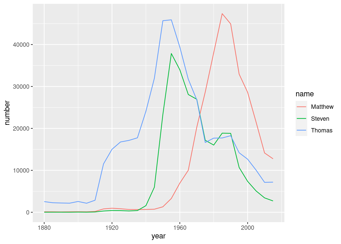
# Calculate the fraction of people born each year with the same name
babynames %>%
  group_by(year) %>%
  mutate(year_total = sum(number)) %>%
  ungroup() %>%
  mutate(fraction = number / year_total) %>%
  # Find the year each name is most common
  group_by(name) %>%
  slice_max(fraction, n = 1)
## # A tibble: 48,040 × 5
## # Groups: name [48,040]
## year name number year_total fraction
## <dbl> <chr> <int> <int> <dbl>
## 1 2015 Aaban 15 3648781 0.00000411
## 2 2015 Aadam 22 3648781 0.00000603
## 3 2010 Aadan 11 3672066 0.00000300
## 4 2015 Aadarsh 15 3648781 0.00000411
## 5 2010 Aaden 450 3672066 0.000123
## 6 2015 Aadhav 31 3648781 0.00000850
## 7 2015 Aadhavan 5 3648781 0.00000137
## 8 2015 Aadhya 265 3648781 0.0000726
## 9 2010 Aadi 54 3672066 0.0000147
## 10 2005 Aadil 20 3828460 0.00000522
## # … with 48,030 more rowsbabynames %>%
# Add columns name_total and name_max for each name
group_by(name) %>%
mutate(name_total = sum(number),
name_max = max(number)) %>%
# Ungroup the table
ungroup() %>%
# Add the fraction_max column containing the number by the name maximum
mutate(fraction_max = number / name_max)## # A tibble: 332,595 × 6
## year name number name_total name_max fraction_max
## <dbl> <chr> <int> <int> <int> <dbl>
## 1 1880 Aaron 102 114739 14635 0.00697
## 2 1880 Ab 5 77 31 0.161
## 3 1880 Abbie 71 4330 445 0.160
## 4 1880 Abbott 5 217 51 0.0980
## 5 1880 Abby 6 11272 1753 0.00342
## 6 1880 Abe 50 1832 271 0.185
## 7 1880 Abel 9 10565 3245 0.00277
## 8 1880 Abigail 12 72600 15762 0.000761
## 9 1880 Abner 27 1552 199 0.136
## 10 1880 Abraham 81 17882 2449 0.0331
## # … with 332,585 more rowsnames_normalized <- babynames %>%
group_by(name) %>%
mutate(name_total = sum(number),
name_max = max(number)) %>%
ungroup() %>%
mutate(fraction_max = number / name_max)
names_filtered <- names_normalized %>%
# Filter for the names Steven, Thomas, and Matthew
filter(name %in% c("Steven", "Thomas", "Matthew"))
# Visualize these names over time
ggplot(names_filtered, aes(year, fraction_max, color = name)) + geom_line()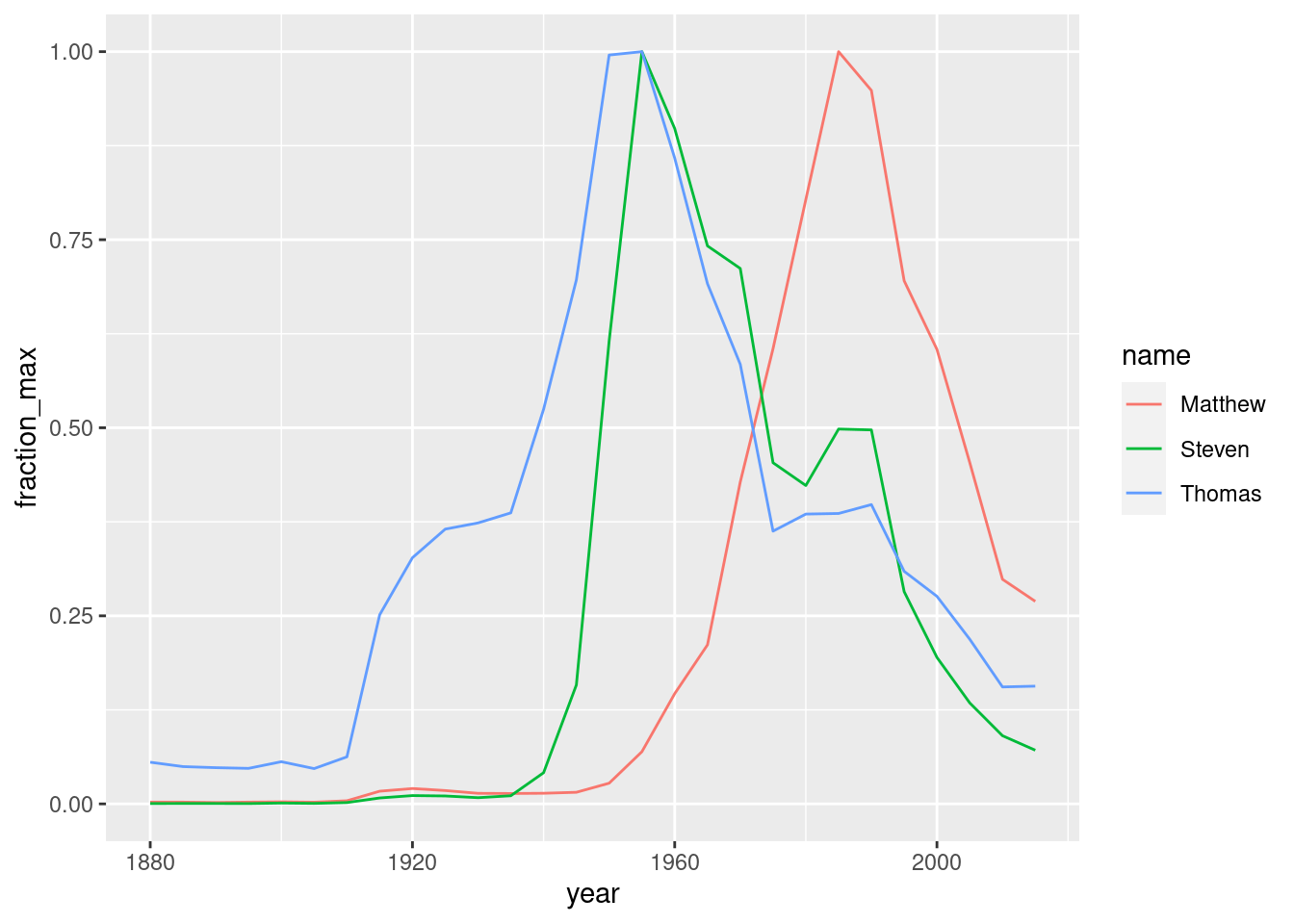
babynames_fraction <- babynames %>%
  group_by(year) %>%
    mutate(year_total = sum(number)) %>%
      ungroup() %>%
        mutate(fraction = number / year_total)

babynames_fraction %>%
  # Arrange the data in order of name, then year
  arrange(name, year) %>%
  # Group the data by name
  group_by(name) %>%
  # Add a ratio column that contains the ratio of fraction between each year
  mutate(ratio = fraction / lag(fraction))
## # A tibble: 332,595 × 6
## # Groups: name [48,040]
## year name number year_total fraction ratio
## <dbl> <chr> <int> <int> <dbl> <dbl>
## 1 2010 Aaban 9 3672066 0.00000245 NA
## 2 2015 Aaban 15 3648781 0.00000411 1.68
## 3 1995 Aadam 6 3652750 0.00000164 NA
## 4 2000 Aadam 6 3767293 0.00000159 0.970
## 5 2005 Aadam 6 3828460 0.00000157 0.984
## 6 2010 Aadam 7 3672066 0.00000191 1.22
## 7 2015 Aadam 22 3648781 0.00000603 3.16
## 8 2010 Aadan 11 3672066 0.00000300 NA
## 9 2015 Aadan 10 3648781 0.00000274 0.915
## 10 2000 Aadarsh 5 3767293 0.00000133 NA
## # … with 332,585 more rowsbabynames_ratios_filtered <- babynames_fraction %>%
arrange(name, year) %>%
group_by(name) %>%
mutate(ratio = fraction / lag(fraction)) %>%
filter(fraction >= 0.00001)
babynames_ratios_filtered %>%
# Extract the largest ratio from each name
slice_max(ratio, n = 1) %>%
# Sort the ratio column in descending order
arrange(desc(ratio)) %>%
# Filter for fractions greater than or equal to 0.001
filter(fraction >= 0.001)## # A tibble: 291 × 6
## # Groups: name [291]
## year name number year_total fraction ratio
## <dbl> <chr> <int> <int> <dbl> <dbl>
## 1 1960 Tammy 14365 4152075 0.00346 70.1
## 2 2005 Nevaeh 4610 3828460 0.00120 45.8
## 3 1940 Brenda 5460 2301630 0.00237 37.5
## 4 1885 Grover 774 240822 0.00321 36.0
## 5 1945 Cheryl 8170 2652029 0.00308 24.9
## 6 1955 Lori 4980 4012691 0.00124 23.2
## 7 2010 Khloe 5411 3672066 0.00147 23.2
## 8 1950 Debra 6189 3502592 0.00177 22.6
## 9 2010 Bentley 4001 3672066 0.00109 22.4
## 10 1935 Marlene 4840 2088487 0.00232 16.8
## # … with 281 more rows