7 Leaflet Maps
Main functions and concepts covered in this BP chapter:
get_acs()leaflet()
Packages used in this chapter:
## Load all packages used in this chapter
library(tidyverse) #includes dplyr, ggplot2, and other common packages
## ── Attaching packages ─────────────────────────────────────── tidyverse 1.3.2 ──
## ✔ ggplot2 3.4.0 ✔ purrr 0.3.5
## ✔ tibble 3.1.8 ✔ dplyr 1.0.10
## ✔ tidyr 1.2.1 ✔ stringr 1.5.0
## ✔ readr 2.1.3 ✔ forcats 0.5.2
## ── Conflicts ────────────────────────────────────────── tidyverse_conflicts() ──
## ✖ dplyr::filter() masks stats::filter()
## ✖ dplyr::lag() masks stats::lag()library(tidycensus)
library(viridis)## Loading required package: viridisLiteDatasets used in this chapter:
## Load datasets used in this chapter#census_api_key("ca24a38ee3604f744dbdf2e64bc93a3ac214a7d7")Some of you might find it helpful to check out DataCamp’s Leaflet course, but it is not assigned. They also have other courses on spatial data). If you do any (or parts of…you don’t need to do entire courses, other than the ones I assigned) of these DC courses, you are free to add notes to this chapter, but I won’t be looking for that when checking off this chapter. Instead, this chapter will be based off the tutorial I give you and your own notes.
For two of the projects, you will be required to make maps (optional for the RP). I will give you a separate GitHub repo to help you learn how to make interactive maps using https://rstudio.github.io/leaflet. For this BP chapter, you will write your own short tutorial on how to make a leaflet map. You can copy/paste from what I give you and what we discuss as part of the course. You are also free to use content from the internet or the DataCamp course on leaflet (but as mentioned above, these notes are meant to be your own tutorial, not something that just follows the DC course).
So what should this chapter include? Suppose in a year you want to make a leaflet map, but you don’t remember anything about how to do so. You should be able to open up this chapter and follow along to create an interactive map using leaflet. Include enough details so you understand what’s going on, but not more than you think will be helpful. I might give you 8 maps in my tutorial, but that doesn’t mean yours should include 8 maps (in fact, I suggest only including one or two since otherwise the file size might get too big for GitHub). Since no two people find the same explanations/examples equally clear, I don’t expect multiple people in the class to have the same chapter (and won’t give credit if that’s what I find). You can talk to each other, but write your own.
This chapter might be graded somewhat differently from the previous chapters.
7.0.1 get_acs
The following link goes through the different arguments of get_acs. To get variables, you have to find their code instead of their name. To do this, use the load_variables() function. The function takes two required arguments: the year of the Census or endyear of the ACS sample, and the dataset name, which varies in availability by year. Once you view the dataset, you can use the filter option in the top left corner to search for specific variables. Make sure to pay attention to the geography column, as different variables have different labels for geography.
v20 <- load_variables(2020, "acs5", cache = TRUE)

View(v20)
## Warning in View(v20): unable to open displayERROR: in .External2(C_dataviewer, x, title): unable to start data viewer
You can also rename variables by what their actual name is rather than their code.
texaspop <- get_acs(geography = "tract", variables = (population = "B01003_001"),
                state = "TX", geometry = TRUE, year = 2020)
## Getting data from the 2016-2020 5-year ACS## Warning: • You have not set a Census API key. Users without a key are limited to 500
## queries per day and may experience performance limitations.
## ℹ For best results, get a Census API key at
## http://api.census.gov/data/key_signup.html and then supply the key to the
## `census_api_key()` function to use it throughout your tidycensus session.
## This warning is displayed once per session.## Downloading feature geometry from the Census website. To cache shapefiles for use in future sessions, set `options(tigris_use_cache = TRUE)`.##
|
| | 0%
|
| | 1%
|
|= | 1%
|
|= | 2%
|
|== | 2%
|
|== | 3%
|
|=== | 4%
|
|=== | 5%
|
|==== | 5%
|
|==== | 6%
|
|===== | 7%
|
|===== | 8%
|
|====== | 8%
|
|====== | 9%
|
|======= | 9%
|
|======= | 10%
|
|======== | 11%
|
|========= | 12%
|
|========= | 13%
|
|========== | 14%
|
|========== | 15%
|
|=========== | 15%
|
|=========== | 16%
|
|============ | 17%
|
|============= | 18%
|
|============== | 19%
|
|============== | 20%
|
|=============== | 21%
|
|================ | 22%
|
|================= | 24%
|
|================== | 25%
|
|=================== | 27%
|
|==================== | 28%
|
|===================== | 29%
|
|====================== | 32%
|
|======================= | 33%
|
|========================= | 36%
|
|========================== | 36%
|
|================================ | 45%
|
|==================================== | 51%
|
|==================================== | 52%
|
|===================================== | 53%
|
|======================================== | 57%
|
|============================================ | 62%
|
|=============================================== | 68%
|
|================================================ | 69%
|
|=================================================== | 73%
|
|==================================================== | 74%
|
|==================================================== | 75%
|
|===================================================== | 76%
|
|======================================================= | 78%
|
|======================================================= | 79%
|
|======================================================== | 80%
|
|========================================================== | 83%
|
|=========================================================== | 84%
|
|============================================================ | 85%
|
|=============================================================== | 90%
|
|=================================================================== | 95%
|
|======================================================================| 100%ggplot(texaspop, aes(fill = estimate, color = estimate)) +
geom_sf() +
coord_sf(crs = 26914) +
scale_fill_viridis(option = "magma") +
scale_color_viridis(option = "magma")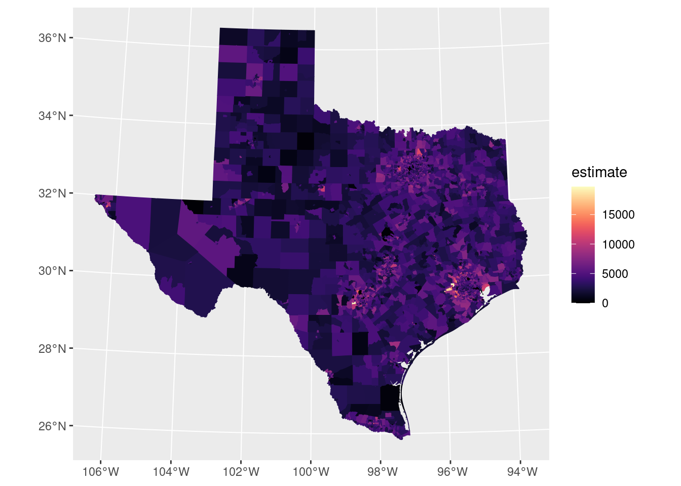
library(tidyverse)
library(leaflet)
library(rmapshaper)
library(tidycensus)
options(tigris_use_cache = TRUE)

## turn off scientific notation
options(scipen = 999)


## Download GIS data for maps
##   geometry = TRUE --> include GIS shapefile data to create maps
##   B01001_001: total population
##   NOTE: When you download the county data for the regressions, use options: geometry = False, keep_geo_vars = FALSE

# Median household income
countyGIS <- get_acs(geography = "county",
              variables = "B01001_001",
              geometry = TRUE,
              keep_geo_vars = TRUE)

# State data (for displaying state borders on map)
stateGIS <- get_acs(geography = "state",
              variables = "B01001_001",
              geometry = TRUE,
              keep_geo_vars = FALSE)
countyGISsave <- countyGIS
stateGISsave <- stateGISstateGIS <- stateGISsave
countyGIS <- countyGISsave
## Simplify GIS data to make file sizes smaller. This essentially removes some details along coastlines and very-not-straight borders.
stateGIS <- ms_simplify(stateGIS, keep = 0.01)
countyGIS <- ms_simplify(countyGIS, keep = 0.01)
countyGIS <- countyGIS %>%
select(FIPS = GEOID,
stFIPS = STATEFP,
coFIPS = COUNTYFP,
coNAME = NAME.x,
pop = estimate,
geometry)
## For mapping, let's drop the following:
## Puerto Rico (ST FIPS 72) (no election data)
## Alaska (ST FIPS 02) (voting data isn't reported by county...we could also map the legislative districts, but we're not going to since we'd rather have smaller maps without those extra details)
## Hawaii (ST FIPS 15) (so our map can zoom in on continental 48 states)
countyGIS <- countyGIS %>% filter(stFIPS != "72" & stFIPS != "02" & stFIPS != "15")
stateGIS <- stateGIS %>% filter(GEOID != "72" & GEOID != "02" & GEOID != "15")
## join 2-character state abbreviation and create name = "county, St" for labeling maps (e.g., Outagamie, WI)
fipsToSTcode <- fips_codes %>% select(stFIPS = state_code, stNAME = state) %>% unique()
countyGIS <- inner_join(countyGIS,fipsToSTcode,by="stFIPS")
countyGIS <- countyGIS %>% mutate(name = paste0(coNAME,", ", stNAME))
## NOTE: If you don't use keep_geo_vars = TRUE, you don't get separate STATEFP and COUNTYFP, but you can use mutate() and create stFIPS = substr(GEOID,1,2) and coFIPS = substr(GEOID,3,5)7.0.2 Election Data
Now we’re going to download 2020 county-level election results from a GitHub repo. You can read more about the data in the repo.
## 2020 Election data
dta2020 <- read_csv("https://raw.githubusercontent.com/tonmcg/US_County_Level_Election_Results_08-20/master/2020_US_County_Level_Presidential_Results.csv")

## Calculate percentages based on total votes for Trump and Biden (GOP and Dem) only
##   In some years there have been ties, so we're allowing for that
##   stdVotes and stdVotesLog will be used to scale color opacity from 0 to 1 based on total votes

dta2020 <- dta2020 %>%
            mutate(pctGOP = votes_gop/(votes_gop + votes_dem),
                   totalVotes = votes_gop + votes_dem,
                   winner = ifelse(dta2020$votes_gop > dta2020$votes_dem,"Trump",
                                   ifelse(dta2020$votes_gop < dta2020$votes_dem,"Biden",
                                          "Tie")),
                   pctWinner = ifelse(dta2020$votes_gop > dta2020$votes_dem,pctGOP,1-pctGOP),
                   FontColorWinner = ifelse(dta2020$votes_gop > dta2020$votes_dem,"red",
                                      ifelse(dta2020$votes_gop < dta2020$votes_dem,"blue",
                                             "purple")),
                   pctGOPcategories = ifelse(pctGOP<0.48,"0-48%",
                                             ifelse(pctGOP<0.5,"48-50%",
                                                    ifelse(pctGOP<0.52, "50-52%",
                                                           "52-100%"))),
                   stdVotes = (totalVotes-min(totalVotes))/(max(totalVotes)-min(totalVotes)),
                   stdVotesLog = (log(totalVotes)-min(log(totalVotes)))/(max(log(totalVotes))-min(log(totalVotes)))
                   )


dta2020 <- dta2020 %>%
            select(FIPS =  county_fips, pctGOP, totalVotes, winner, pctWinner, pctGOPcategories, FontColorWinner, stdVotes, stdVotesLog)
## merge GIS data with voting data using FIPS code
countyGISelection <- left_join(countyGIS,dta2020,by="FIPS")7.0.3 Creating Pop-Up Labels
# county name (zip code)
# winner of county in the color of the winner and percentage of votes won
# total votes in county

popupLabels <- paste0("<b>",countyGISelection$name," (",countyGISelection$FIPS,")</b>",
                    "<br><font color='",countyGISelection$FontColorWinner,"'>",countyGISelection$winner,
                    ": ",
                    format(countyGISelection$pctWinner*100,digits=4, trim=TRUE),
                    "%</font>",
                    "<br>Total votes: ", format(countyGISelection$totalVotes,big.mark=",", trim=TRUE)) %>%
              lapply(htmltools::HTML)
7.0.4 Creating Graphic
## create color palette used by map

# "n =" is the number of bins
# we can either have evenly spaced bins or use n = c(0,0.2,0.3,.4,.45,.49,.51,.55,.6,0.7,0.8, 1) to create custom spacing (can input own numbers obviously)

pal <- colorBin("RdBu", countyGISelection$pctGOP, n = , reverse=TRUE)
One of the arguments of leaflet() is leafletOptions(crsClass = ). CRS stands for coordinate reference system, a term used by geographers to explain what the coordinates mean in a coordinate vector. L.CRS.EPSG3857 is the most common and should be the default.
# leaflet(dataset, leafletOptions(crsClass = ), width = "width you want graphic%") <- usually just do 100% unless you need it to be bigger/smaller

leaflet(countyGISelection, options = leafletOptions(crsClass = "L.CRS.EPSG3857"), width="100%") %>%

  # add the outlines of the county, can specify thickness (weight =), color, and opacity
  addPolygons(weight = 0.9, color = "white", opacity = 0.2,

    # add in the fill color for the counties that you already created along with the variable that it represents
    fillColor = ~pal(pctGOP), fillOpacity = 1, smoothFactor = 0.5,

    #add popupLabels
    label = popupLabels,
    labelOptions = labelOptions(direction = "auto")) %>%

    #add state borders
    addPolygons(data = stateGIS,fill = FALSE,color="black",weight = 1) %>%

    #add legend
    addLegend(pal = pal,values = ~countyGISelection$pctGOP, opacity = 0.7, title = "% Trump",position = "bottomright")
## Warning: sf layer has inconsistent datum (+proj=longlat +datum=NAD83 +no_defs).
## Need '+proj=longlat +datum=WGS84'
## Warning: sf layer has inconsistent datum (+proj=longlat +datum=NAD83 +no_defs).
## Need '+proj=longlat +datum=WGS84'Instead of bins you can use a continuous scale. The map below uses a continuous scale with 2 colors. The two colors, red and blue, become become purple in the middle where they mix. You could also do a 3 color scale and add another color, like white, in between red and blue. Instead of purple, you would have white where the votes are pretty evenly split.
pal <- colorNumeric(
  palette = colorRampPalette(c('red', 'blue'))(length(countyGISelection$pctGOP)),
  domain = countyGISelection$pctGOP, reverse=TRUE)

leaflet(countyGISelection, options = leafletOptions(crsClass = "L.CRS.EPSG3857"), width="100%") %>%
  addPolygons(weight = 0.5, color = "gray", opacity = 0.7,
    fillColor = ~pal(pctGOP), fillOpacity = 1, smoothFactor = 0.5,
    label = popupLabels,
    labelOptions = labelOptions(direction = "auto")) %>%
    addPolygons(data = stateGIS,fill = FALSE,color="black",weight = 1) %>%
    addLegend(pal = pal,values = ~countyGISelection$pctGOP, opacity = 0.7, title = "% Trump",position = "bottomright")
This map uses 4 custom-labeled factors. This map is similar to what you often see on the news, displaying either red or blue. However, this one highlights close counties in slightly different colors. As you can see, there aren’t very many close counties (something that’s impossible to see on a two-color map).
pal <- colorNumeric(
  palette = colorRampPalette(c('red', 'white', 'blue'))(length(countyGISelection$pctGOP)),
  domain = countyGISelection$pctGOP, reverse=TRUE)

factorPal <- colorFactor(c("blue", "cyan", "magenta", "red"), countyGISelection$pctGOPcategories )

leaflet(countyGISelection, options = leafletOptions(crsClass = "L.CRS.EPSG3857"), width="100%") %>%
  addPolygons(weight = 0.5, color = "gray", opacity = 0.7,
    fillColor = ~factorPal(pctGOPcategories), fillOpacity = 1, smoothFactor = 0.5,
    label = popupLabels,
    labelOptions = labelOptions(direction = "auto")) %>%
    addPolygons(data = stateGIS,fill = FALSE,color="black",weight = 1) %>%
    addLegend(pal = factorPal,values = ~countyGISelection$pctGOPcategories, opacity = 0.7, title = "% Trump",position = "bottomright")
7.0.5 Median Income
Now we’ll create a map that shows the median income of each county. First we need to pull in the data from the census data.
countyincome <- get_acs(geography = "county",
              variables = "B07411_001",
              keep_geo_vars = TRUE)
## Getting data from the 2017-2021 5-year ACScountyincome <- countyincome %>%
select(FIPS = GEOID,
COUNTY = NAME,
median_income = estimate)
countyincome## # A tibble: 3,221 × 3
## FIPS COUNTY median_income
## <chr> <chr> <dbl>
## 1 01001 Autauga County, Alabama 29733
## 2 01003 Baldwin County, Alabama 31323
## 3 01005 Barbour County, Alabama 19813
## 4 01007 Bibb County, Alabama 23520
## 5 01009 Blount County, Alabama 28027
## 6 01011 Bullock County, Alabama 21580
## 7 01013 Butler County, Alabama 22335
## 8 01015 Calhoun County, Alabama 25835
## 9 01017 Chambers County, Alabama 23855
## 10 01019 Cherokee County, Alabama 25537
## # … with 3,211 more rowsstateGIS <- stateGISsave
countyGIS <- countyGISsave
## Simplify GIS data to make file sizes smaller. This essentially removes some details along coastlines and very-not-straight borders.
stateGIS <- ms_simplify(stateGIS, keep = 0.01)
countyGIS <- ms_simplify(countyGIS, keep = 0.01)
countyGIS <- countyGIS %>%
select(FIPS = GEOID,
stFIPS = STATEFP,
coFIPS = COUNTYFP,
coNAME = NAME.x,
pop = estimate,
geometry)
## For mapping, let's drop the following:
## Puerto Rico (ST FIPS 72) (no election data)
## Alaska (ST FIPS 02) (voting data isn't reported by county...we could also map the legislative districts, but we're not going to since we'd rather have smaller maps without those extra details)
## Hawaii (ST FIPS 15) (so our map can zoom in on continental 48 states)
countyGIS <- countyGIS %>% filter(stFIPS != "72" & stFIPS != "02" & stFIPS != "15")
stateGIS <- stateGIS %>% filter(GEOID != "72" & GEOID != "02" & GEOID != "15")
## join 2-character state abbreviation and create name = "county, St" for labeling maps (e.g., Outagamie, WI)
fipsToSTcode <- fips_codes %>% select(stFIPS = state_code, stNAME = state) %>% unique()
countyGIS <- inner_join(countyGIS,fipsToSTcode,by="stFIPS")
countyGIS <- countyGIS %>% mutate(name = paste0(coNAME,", ", stNAME))
## NOTE: If you don't use keep_geo_vars = TRUE, you don't get separate STATEFP and COUNTYFP, but you can use mutate() and create stFIPS = substr(GEOID,1,2) and coFIPS = substr(GEOID,3,5)countyGISincome <- left_join(countyGIS,countyincome,by="FIPS")
head(countyGISincome)## Simple feature collection with 6 features and 9 fields
## Geometry type: MULTIPOLYGON
## Dimension: XY
## Bounding box: xmin: -111.6345 ymin: 39.04326 xmax: -91.5291 ymax: 45.61104
## Geodetic CRS: NAD83
## FIPS stFIPS coFIPS coNAME pop stNAME name
## 1 20161 20 161 Riley 72602 KS Riley, KS
## 2 19159 19 159 Ringgold 4739 IA Ringgold, IA
## 3 30009 30 009 Carbon 10488 MT Carbon, MT
## 4 16007 16 007 Bear Lake 6327 ID Bear Lake, ID
## 5 55011 55 011 Buffalo 13314 WI Buffalo, WI
## 6 31185 31 185 York 14164 NE York, NE
## COUNTY median_income geometry
## 1 Riley County, Kansas 26604 MULTIPOLYGON (((-96.95872 3...
## 2 Ringgold County, Iowa 28058 MULTIPOLYGON (((-94.47078 4...
## 3 Carbon County, Montana 30885 MULTIPOLYGON (((-109.7987 4...
## 4 Bear Lake County, Idaho 27500 MULTIPOLYGON (((-111.0467 4...
## 5 Buffalo County, Wisconsin 35320 MULTIPOLYGON (((-91.65025 4...
## 6 York County, Nebraska 34014 MULTIPOLYGON (((-97.82629 4...popupLabels <- paste0("<b>",countyGISincome$name," (",countyGISincome$FIPS,")</b>",
"<br>", "Median Income: ",
"$",countyGISincome$median_income) %>%
lapply(htmltools::HTML)# leaflet(dataset, leafletOptions(crsClass = ), width = "width you want graphic%") <- usually just do 100% unless you need it to be bigger/smaller
pal <- colorNumeric(
palette = colorRampPalette(c('green', 'red'))(length(countyGISincome$median_income)),
domain = countyGISincome$median_income, reverse=TRUE)
leaflet(countyGISincome, options = leafletOptions(crsClass = "L.CRS.EPSG3857"), width="100%") %>%
# add the outlines of the county, can specify thickness (weight =), color, and opacity
addPolygons(weight = 0.9, color = "white", opacity = 0.2,
# add in the fill color for the counties that you already created along with the variable that it represents
fillColor = ~pal(median_income), fillOpacity = 1.8, smoothFactor = 0.5,
#add popupLabels
label = popupLabels,
labelOptions = labelOptions(direction = "auto")) %>%
#add state borders
addPolygons(data = stateGIS,fill = FALSE,color="black",weight = 1) %>%
#add legend
addLegend(pal = pal,values = ~countyGISincome$median_income, opacity = 0.7, title = "Median Income (2020$)",position = "bottomright")## Warning: sf layer has inconsistent datum (+proj=longlat +datum=NAD83 +no_defs).
## Need '+proj=longlat +datum=WGS84'
## Warning: sf layer has inconsistent datum (+proj=longlat +datum=NAD83 +no_defs).
## Need '+proj=longlat +datum=WGS84'medianrent2bed <- get_acs(geography = "tract",
variables = "B25031_004",
keep_geo_vars = TRUE)## Getting data from the 2017-2021 5-year ACSERROR:: Your API call has errors. The API message returned is error: unknown/unsupported geography heirarchy.